What is HNSW? The vector index behind most vector search
HNSW is a layered graph index for approximate nearest neighbor search. How M, ef_construction and ef_search trade recall for speed, with a Python build.

HNSW (Hierarchical Navigable Small World) is a graph index for approximate nearest neighbor search: every vector is a node linked to its close neighbors, and a few randomly chosen nodes also live in sparser upper layers that act as express lanes. A query starts at the top, walks greedily toward the target, drops a layer, and repeats, so it checks a few hundred vectors instead of all of them. Yu. A. Malkov and D. A. Yashunin posted it to arXiv in March 2016, and it is the graph index you will find in pgvector, Qdrant and many other vector stores.
Why do vector databases need an index like HNSW?
Because exact search is a full scan. To find the ten nearest neighbors of a query embedding you compute its distance to every stored vector and keep the best ten. That is fine for 50,000 chunks and painful for 50 million, and it gets worse with dimension count, since every distance touches every coordinate. The HNSW paper puts it bluntly: the naive approach “scales linearly with the number of stored elements”.
Approximate nearest neighbor (ANN) search gives up a little accuracy for a lot of speed. The accuracy you give up is measured as recall: of the true top ten, how many did the index return? The paper defines it the same way, as the ratio of true nearest neighbors found to K. Every ANN index, HNSW included, is a dial between recall and the number of vectors you have to look at. If you are new to the storage side, start with what a vector database is; this post is about the index inside it.
How does HNSW work?
Start with a plain proximity graph. Each vector links to a handful of its nearest neighbors. To search, you pick an entry node, look at its neighbors, move to whichever is closest to the query, and stop when no neighbor is closer. That greedy walk works, but on a flat graph it takes many hops to cross the space, and it can get stuck in a local minimum.
HNSW fixes this with layers, and the paper says the idea is a generalization of the skip list. When a vector is inserted, it draws a random maximum level from an exponentially decaying distribution: l = floor(-ln(uniform(0, 1)) * mL). Almost every node lives only on layer 0. A small fraction also lives on layer 1, a smaller fraction on layer 2, and so on. Upper layers are sparse, so their links are long. Layer 0 is dense, so its links are short.
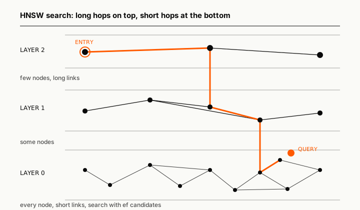
Search has two phases (Algorithm 5 in the paper):
- From the entry point on the top layer, greedily move to the closest neighbor until nothing is closer. Drop to the next layer, starting from that node. Repeat with a candidate list of size one.
- On layer 0, run the same search with a wider candidate list of size
ef, and return the best K from it.
Insertion is the same search, then linking. A new node finds its efConstruction nearest candidates on each layer it belongs to, connects to M of them in both directions, and if a neighbor now has too many links, that neighbor’s list is pruned back. The paper describes a neighbor-selection heuristic that prefers diverse directions over the strictly closest nodes, which keeps the graph connected across clusters.
What do M, ef_construction and ef_search do?
These three names show up in every HNSW implementation, sometimes spelled slightly differently.
- M: links per node on the upper layers. Layer 0 allows
Mmax0, and the paper finds2 * Ma good choice. It suggests a reasonable range of 5 to 48: smaller M suits low recall and low-dimensional data, larger M suits high recall and high-dimensional data. Memory grows with M. - efConstruction: how wide the search is while building. Higher gives a better graph and a slower build. The paper’s test built a good 10M SIFT index with
efConstruction=100, and found that pushing it further added little quality for much longer builds. - ef (called
ef_searchin pgvector,efin Qdrant): how wide the bottom-layer search is at query time. This is the knob you turn in production, per query, without rebuilding anything.
The paper also sets the level multiplier mL to 1/ln(M) as a simple near-optimal choice, which is why most libraries do not expose it.
Defaults differ by product. pgvector uses m = 16, ef_construction = 64 and hnsw.ef_search = 40. Qdrant’s indexing docs show m: 16 and ef_construct: 100, with search-time ef defaulting to ef_construct. I covered the Postgres side in the pgvector tutorial.
What does HNSW look like in code?
I only trust an index once I have built one, so here is HNSW in about 70 lines of standard-library Python. It follows the paper’s Algorithms 1, 2 and 5, with the simple neighbor selection (Algorithm 3) instead of the heuristic, and counts distance computations, which is the cost that matters.
# hnsw.py: a small HNSW index in pure Python 3, no dependencies.
import heapq, math, random

random.seed(7)
DIM, N, M, EF_CONSTRUCTION = 16, 3000, 8, 64
M0, ML = 2 * M, 1 / math.log(M)          # the paper's defaults: Mmax0 = 2M, mL = 1/ln(M)
calls = 0                                 # distance computations, the cost that matters

def dist(a, b):
    global calls
    calls += 1
    return sum((x - y) ** 2 for x, y in zip(a, b))

data = [[random.gauss(0, 1) for _ in range(DIM)] for _ in range(N)]
graph = []          # graph[layer][node] -> list of neighbour ids
entry, top = None, -1

def search_layer(q, eps, ef, layer):
    visited = set(eps)
    cand = [(dist(q, data[e]), e) for e in eps]          # min-heap: closest first
    best = [(-d, e) for d, e in cand]                     # max-heap: furthest first
    heapq.heapify(cand); heapq.heapify(best)
    while cand:
        d, c = heapq.heappop(cand)
        if d > -best[0][0]:
            break                                         # nothing closer left to expand
        for n in graph[layer].get(c, []):
            if n in visited:
                continue
            visited.add(n)
            dn = dist(q, data[n])
            if len(best) < ef or dn < -best[0][0]:
                heapq.heappush(cand, (dn, n)); heapq.heappush(best, (-dn, n))
                if len(best) > ef:
                    heapq.heappop(best)
    return sorted((-d, e) for d, e in best)

def insert(i):
    global entry, top
    level = int(-math.log(1 - random.random()) * ML)      # exponentially decaying level
    while len(graph) <= level:
        graph.append({})
    for l in range(level + 1):
        graph[l][i] = []
    if entry is None:
        entry, top = i, level
        return
    ep = [entry]
    for l in range(top, level, -1):                       # greedy descent, ef = 1
        ep = [search_layer(data[i], ep, 1, l)[0][1]]
    for l in range(min(level, top), -1, -1):
        found = search_layer(data[i], ep, EF_CONSTRUCTION, l)
        cap = M0 if l == 0 else M
        graph[l][i] = [e for _, e in found[:M]]
        for e in graph[l][i]:                             # bidirectional links, then shrink
            graph[l][e].append(i)
            if len(graph[l][e]) > cap:
                graph[l][e] = sorted(graph[l][e], key=lambda n: dist(data[e], data[n]))[:cap]
        ep = [e for _, e in found]
    if level > top:
        entry, top = i, level

def knn(q, k, ef):
    ep = [entry]
    for l in range(top, 0, -1):
        ep = [search_layer(q, ep, 1, l)[0][1]]
    return [e for _, e in search_layer(q, ep, max(ef, k), 0)[:k]]

for i in range(N):
    insert(i)
print(f"{N} vectors, {DIM} dims, M={M}, layers={top + 1}, "
      f"nodes per layer={[len(g) for g in graph]}")

queries = [[random.gauss(0, 1) for _ in range(DIM)] for _ in range(50)]
truth = []
calls = 0
for q in queries:
    truth.append(set(sorted(range(N), key=lambda j: dist(q, data[j]))[:10]))
print(f"brute force  recall@10 1.000  distance calls per query {calls // len(queries)}")
for ef in (10, 20, 40, 80, 160):
    calls, hits = 0, 0
    for q, t in zip(queries, truth):
        hits += len(set(knn(q, 10, ef)) & t)
    print(f"HNSW ef={ef:<4} recall@10 {hits / (10 * len(queries)):.3f}  "
          f"distance calls per query {calls // len(queries)}")
Output (Python 3.9.6):
3000 vectors, 16 dims, M=8, layers=4, nodes per layer=[3000, 393, 53, 3]
brute force  recall@10 1.000  distance calls per query 3000
HNSW ef=10   recall@10 0.692  distance calls per query 159
HNSW ef=20   recall@10 0.860  distance calls per query 240
HNSW ef=40   recall@10 0.952  distance calls per query 379
HNSW ef=80   recall@10 0.986  distance calls per query 609
HNSW ef=160  recall@10 0.994  distance calls per query 955
Two things to read off this. The layer sizes fall by roughly a factor of M each time (3,000, 393, 53, 3), which is the exponential level distribution doing its job. And ef is a clean dial: at ef=40, the pgvector default, this toy index finds 95% of the true top ten while computing distances to about an eighth of the data. At ef=160 it reaches 99.4% for about a third. Random Gaussian vectors in 16 dimensions are a hard, unclustered case; real embeddings have more structure, and the ratio gets far better as N grows, because the search cost grows roughly with log N and the scan grows with N.
Where does HNSW break?
Memory. HNSW keeps the full vectors plus the link lists, and it wants them in RAM. pgvector’s README says HNSW “has slower build times and uses more memory” than IVFFlat, in exchange for a better speed-recall trade-off. For a large corpus, the index often costs more than the database it sits in. Shorter vectors help, which is one argument for Matryoshka embeddings and for halfvec.
Filters. An HNSW search returns ef candidates; a WHERE tenant_id = 42 clause then throws most of them away. pgvector’s docs give the arithmetic: with a filter matching 10% of rows and the default ef_search of 40, you get about 4 rows on average. Qdrant attacks this by adding filter-aware edges to the graph, and warns that combining two or more strict filters “might still lead to disconnected graph components.”
Deletes and updates. Removing a node punches a hole in other nodes’ neighbor lists. Qdrant’s docs list soft-deleted points as another cause of disconnected graph components. With heavy churn, plan for periodic rebuilds.
Silent recall loss. Nothing errors when recall drops. The only way to know is to compare against exact search on a sample of real queries, which pgvector suggests doing by turning off index scans inside a transaction. I would put that check in CI for any retrieval system.
HNSW vs IVF: which should I use?
IVF (inverted file) clusters vectors with k-means and searches only the clusters nearest the query. It builds faster, uses less memory, and needs data to train its clusters first. HNSW has no training step, so you can create the index on an empty table, and it gives better recall per millisecond. pgvector’s README states both trade-offs. My default is HNSW until memory becomes the constraint, then IVF with product quantization, such as the IVFPQ index in FAISS that the ColBERT authors used for end-to-end retrieval.
What I would do
From a data-platform seat, the line I would circle is that an ANN index is a cache with a recall SLA, and nobody writes the SLA down. So:
- Start with exact search. Under a few hundred thousand vectors it is often fast enough, and recall is 1.0 by definition.
- When you add HNSW, keep the library defaults for
Mandef_construction, and tuneef_searchper query against a labelled set. It is the only knob you can change without a rebuild. - Log recall@10 against brute force on a nightly sample. If it drifts after a bulk load or a wave of deletes, rebuild.
- Test filtered queries separately. They are where HNSW quietly returns three rows instead of ten.
- Pair it with keyword search. HNSW finds near vectors, and near vectors miss exact identifiers; hybrid search covers that gap.
FAQ
What does HNSW stand for?
Hierarchical Navigable Small World. “Navigable small world” refers to graphs where greedy routing reaches any node in few hops; “hierarchical” refers to the stacked layers with longer links at the top.
Is HNSW exact or approximate?
Approximate. It can miss some true nearest neighbors, and recall depends on M, ef_construction and especially ef_search. Set ef high enough and recall approaches 1.0 at a higher query cost.
What is a good value for ef_search?
Start at the library default (40 in pgvector) and raise it until recall on your own labelled queries stops improving. It must be at least as large as K, and it should be higher still when queries carry selective filters.
How much memory does an HNSW index use?
Roughly the raw vectors plus a neighbor list per node: about M links on upper layers and 2 * M on layer 0, as the paper recommends. The vectors usually dominate, so dimension count and precision matter more than M.
Who invented HNSW?
Yu. A. Malkov and D. A. Yashunin, first posted to arXiv on 30 March 2016 and last revised in August 2018. It extends the earlier Navigable Small World (NSW) graphs, which the paper cites as its starting point.
Sources
- Malkov and Yashunin, Efficient and robust approximate nearest neighbor search using Hierarchical Navigable Small World graphs, arXiv, March 2016 (v4 August 2018)
- pgvector README, version 0.8.7, checked 2026-10-31
- Qdrant, Indexing concepts, checked 2026-10-31
- Johnson, Douze and Jégou, Billion-scale similarity search with GPUs, arXiv, February 2017